Basic Concepts

Reinforcement learning (RL) has been used to solve the interaction problem between agents and environments. The interaction process can be simply described as follows: An agent receives observation from the environment, and acts accordingly. The environment will change due to the action taken by the agent and send a reward to the agent. This process runs repeatedly and the goal of the agent is to maximize the cumulative reward (sum of (discounted) rewards) received. The objective of reinforcement learning is to enable agents to learn strategies which we call ‘policy’ and maximize the cumulative reward.

To have a basic understanding for reinforcement learning, we explain the following basic concepts：

• Markov Decision Processes

• State and action spaces

• Policy

• Trajectory

• Return and reward

To understand reinforcement learning better, we further explain the following concepts:

• RL optimization problem

• Value function

• Policy gradients

• Actor Critic

• Model-based RL

In the end, we will list and answer some common questions raised in the domain of reinforcement learning for reference.

Markov Decision Process/MDP

Markov Decision Process (MDP) is the ideal mathematical model of reinforcement learning and the commonest one.

• Markov property：State \(s_t\) is Markov, iff \(P[s_{t+1}|s_t] = P[s_{t+1}|s_1, ..., s_t]\) .

• A Markov process is a memoryless random process, i.e., a sequence of random states \(S_1\),　\(S_2\)… with the Markov process.

• Markov process is a binary tuple \((S, P)\) , satisfying: \(S\) a finite set of states, \(P\) is a probability transition matrix. There are no rewards or actions in a Markov process. A Markov process that takes actions and rewards into account is called an MDP.

• MDP is a tuple \((S, A, P, R, \gamma)\)， \(S\) is a finite set of states, \(A\) is a finite set of actions， \(P\) is a state transition probability matrix, \(R\) is a reward function， \(\gamma\) is a discount factor used to calculate the accumulated rewards. Unlike the Markov process, the state transfer probability of the Markov decision process is \(P(s_{t+1}|s_t, a_t)\) . \(P(s_{t+1}|s_t, a_t)\) .

• The goal of reinforcement learning is to seek an optimal policy based on an MDP. The so-called policy \(\pi(a|s)\) refers to the mapping of states to actions. In reinforcement learning, we only discuss Markov decision processes with finite state space.

Common methods for solving MDP problems:

1. Dynamic programming (DP) is an optimization method that can compute the optimal policy given an MDP. However, for reinforcement learning problems, traditional DP is of limited use and prone to dimensional catastrophe problems.

   DP has the following characteristics:

   • Updating is based on currently existing estimates: the value estimate of a current state is updated with the value estimate of each of its subsequent states

   • Asymptotic convergence

   • Advantages: reduced variance and faster learning

   • Disadvantages: bias dependent on the quality of the function approximation

2. Monte Carlo methods (MC) are based directly on the definition of the optimal value function and provide an unbiased estimate of the optimal value function by sampling. MC replaces the actual expected return with the sample return and solves the optimal strategy empirically only.

   MC does not need an environmental model. Data simulation and sampling models can be applied to MC and MC can only evaluate a certain state of interest. In comparison with DP, MC performs better when the Markov property does not hold.

3. Temperal-Differnece learning (TD), TD error: \(\delta_{t} = R_{t+1} + \gamma V(S_{t+1}) - V(S_t)\)

   Comparison between TD and MC: The target for MC is \(G_t\), namely, the real return from time t onwards. However, the target for TD (single step TD, TD(0)) is \(R_{t+1} + \gamma V(S_{t+1})\) .

State Spaces

State \(s\) is a global description of the environment，observation \(o\) is a partial description of the environment. States and observations from an environment can be represented by real vectors, matrices or tensors. For example, RGB pictures are used in Atari games to represent information about the game environment, and vectors are used in MuJoCo control tasks to represent the state of an intelligent body.

When an agent can receive all information of states in an environment \(s\) ，we call its learning process fully observable. When an agent can only receive partial information of states in an environment \(o\)，we call its learning process partially observable，namely, partially observable Markov decision processes (POMDP) \((O, A, P, R, \gamma)\).

Action Spaces

Different environments allow different action spaces. The set of all valid actions \(a\) in an environment is generally referred to as the Action Space. The action space can be classified into a discrete action space or a continuous action space.

For example, in Atari games and SMAC games, the action spaces are both discrete and only a limited number of actions can be selected from each space. However, in some robot continuous control tasks such as MuJoCo, the action space is continuous and generally belongs to a real-valued vector interval.

Policy

Policy determines actions an agent takes when facing different states. If a policy is deterministic, it is usually denoted by \(a_t = \mu(s_t)\) . when a policy is stochastic，it is usually denoted by \(a_t ~ \pi(·｜s_t')\).

In reinforcement learning，the policy gradient approach requires learning a parametric representation of the policy (parameterized policy) by fitting a policy function with parameters. \(\theta\) is often used as the parameters. Another approach based on value functions does not necessarily require a policy gradient function. In the following sections, we describe in a more detailed approach to learning policies in reinforcement learning.

Trajectory

In reinforcement learning, a sample learning sequence in an MDP is called trajectory \((s_0, a_0, ..., s_n, a_n)\). Trajectory data includes a state transition function，namely, \(s_{t+1} = f(s_t, a_t)\) and a policy followed by the agents. Reinforcement learning contains two parts: how to use the policy to sample the trajectory data and how to use the trajectory data to update the learning target. The difference between the two components creates a difference in reinforcement learning methods.

As the trajectory also contains information about the dynamics of the model in the environment, it is possible to use the policy data to learn information about the environment as well, which can be used to help the learning of the intelligence.

Note that the transition function can be deterministic or stochastic. In a grid world, the transition function is deterministic, i.e., an agent is going to go to a certain state given its current state and action. On the contrary, the state function is stochastic if an agent’s current state and action are given, but the agent may end up with more than one state with each probability smaller than one. A stochastic state function is random in nature and cannot be determined completely by an agent. This case can be easily illustrated in a simple MDP environment.

Return and reward

Reward is a learning signal assigned to an agent by its surrounding environment. When the environment changes，the reward function also changes. The reward function is determined by the current state and the action taken by the agent，and can be written as \(r_t = R(s_t, a_t)\)

Cumulative Reward is the sum of the decaying returns from moment t onwards in an MDP.

\(G_t = R_{t}+\gamma * R_{t+1}+{\gamma}^2 * R_{t+2}+ ...\)

\(\gamma\) The discount factor reflects the ratio between the value of future rewards and that at the present moment. A value close to 0 indicates a tendency towards a ‘myopic’ assessment and a value close to 1 indicates a more forward-looking interest and confidence in the future. The introduction of the discount factor is not only easy to express mathematically, but also avoids falling into an infinite loop and reduces the uncertainty of future benefits.

Other difficulties in dealing with reward functions may exist in different environments, such as sparse rewards where the environment does not give feedback in every state and only acquires rewards after a period of trajectory has elapsed. Therefore, the design and processing of reward functions in reinforcement learning are important directions that have a significant impact on the effectiveness of reinforcement learning.

RL optimization problem

In simple terms, the goal of a reinforcement learning problem is to find a policy that maximizes the expected total reward. Then, if we can calculate the return after each state by taking some action, we only need to take the action with the higher reward or the action that will lead to the states with the higher reward. Thus, the estimation of expected reward is also an optimization direction for reinforcement learning. Another approach is to search directly over the action space. In either case, the ultimate optimization goal is to maximize the reward.

Value functions

State Value Function refers to a long-term expected reward by following a policy \(\pi\) under a state \(s\) . The state value function is one of the criteria for evaluating a policy function

\(V_{\pi}(s) = E_{\pi}[G_t|s_t=s]\)

Action Value Function refers to a long-term expected reward by following a policy \(\pi\) under a state \(s\) , and an action \(a\)

\(Q_{\pi}(s, a) = E_{\pi}[G_t|s_t=s, a_t=a]\)

The relationship between the state-valued function and the action-valued function：

\(V_{\pi}(s) = \sum \pi(a|s)Q_{\pi}(s,a)\)

We can further obtain the relationship between the optimal state value function and the optimal behavioral value function as follows.

\(V*(s)=max_a Q*(s, a)\)

Bellman Equations，The Bellman’s equation is the basis of reinforcement learning. The Bellman equation represents the value of the current state in relation to the value of the next state, and the current reward. We can express the state value function and the action value function as:

\(V_{\pi}(s) = E_{\pi}[R_{t}+\gamma * v_{\pi}(s_{t+1})|s_t=s]\)

\(Q_{\pi}(s, a) = E_{\pi}[R_{t}+\gamma * Q(s_{t+1},a_{t+1})|s_t=s, a_t=a]\)

Bellman Optimality Equations，

\(V*(s)=E[R_{t} + \gamma * max_{\pi}V(s_{t+1})|s_t=s]\)

\(Q*(s, a) = E_{\pi}[R_{t}+\gamma * max_{a'}Q(s_{t+1},a')|s_t=s, a_t=a]\)

Value based reinforcement learning approach includes two steps：policy evaluation and policy improvement. Reinforcement learning first estimate the value function based on the policy，then, improves the policy according to the value function. When the value function reaches the optima, the policy is considered as the optimal policy. This optimal policy is a greedy policy.

For systems where the model is known, the value function can be obtained using DPs; For systems where the model is unknown, it can be obtained using MC or TD.

For a grid reinforcement learning environment，the estimation of the value function is obtained by iteratively updating the table of value functions. In many cases，say, state space and action space are not discrete，the value function cannot be represented by a table. In this situation, we need to take advantage of function approximation to approximate the value function.

Policy Gradients

In some situations, a stochastic policy is better than a deterministic policy. As a result, value-based reinforcement learning cannot learn such policy and a policy-based approach to reinforcement learning is therefore proposed.

Unlike value-based reinforcement learning, policy-based reinforcement learning parameterises the policy and represent it by using linear or non-linear functions to find the optimal parameters that maximize the expectation of the cumulative reward, the goal of reinforcement learning.

In the value-based approach, we iteratively compute the value function and then improve the policy based on the value function, whereas in the policy search approach, we directly compute the policy iteration using policy gradient, i.e. we compute the policy gradient on the action, and iteratively update the policy parameter values along the gradient until the expectation of cumulative return is maximzed, at which point the policy corresponding to the parameter is the optimal policy.

Compared to the value-based approach, the policy gradient reinforcement learning tends to converge to a local minimum, which is not sufficient when evaluating an individual policy and has a large variance.

For a more detailed understanding of the policy based approach, please refer to the specific algorithms in our documentation：　Hands On RL

Actor Critic

Critic, parametrized behavioral value function; performs the value evaluation of the policy.

Actor, parametrized policy function, performs an update of the policy function parameters using the policy gradient according to the value obtained in the Critic part.

In summary, Actor Critic is an approach that learns both the value function and the policy function, combining the advantages of both of these approaches. Various algorithms based on this framework can adapt to problems in different action and state spaces as well as to find optimal policies in different policy spaces.

More Actor Critic algorithms such as A2C, DDPG, TD3, etc. are explained in our documentation.

Model-based RL

Of the above model-free approaches, the value-based approach learns the value function (MC or TD) before updating the policy, while the policy-based approach updates the policy directly. The model-based approach focuses on the environment dynamics, where a model of the environment is learned through sampling, and then the value function/ policy is optimized based on the learned environment model.

Once the modeling of the environment has been completed, there are also two paths in the model-based approach: one is to generate some simulation trajectories from the learned model and estimate the value function from the simulation trajectories to optimise the strategy; the other is to optimize the policy directly from the learned model, which is the route the model-based approach is usually taking. Learning a model of the environment first can help us to solve the problem of sample efficiency in reinforcement learning methods.

The definition of a model can be expressed mathematically as a tuple of state transfer distributions and reward functions.

\(M=(P,R), s_{t+1}\simP(s_{t+1}|s_t, a_t), r_{t}\simR(r_{t}|s_t, a_t)\)

The learning of a model can be extended to different algorithms depending on the model construction.

Model-based policy optimization: A classical approach is to first sample a large amount of data by some strategy, then learn a model to minimize the error, apply the learned model to planning to obtain new data, and repeat the above steps. It is by doing planning on top of the learned model that model-based improves the efficiency of the entire iteration of the reinforcement learning algorithm.

Q&A

Q1: What are model-based and model-free methods，what are the differences？Which category should MC、TD、DP, etc. belong to?

• Answer： model based algorithm means that the algorithm learns the state transition process of the environment and models the environment, whereas a model free algorithm does not require the environment to be modeled. Monte Carlo and TD algorithms are model-free because they do not require the algorithm to model a specific environment. Dynamic programming, on the other hand, is model-based, as the use of dynamic programming requires a complete model of the environment.

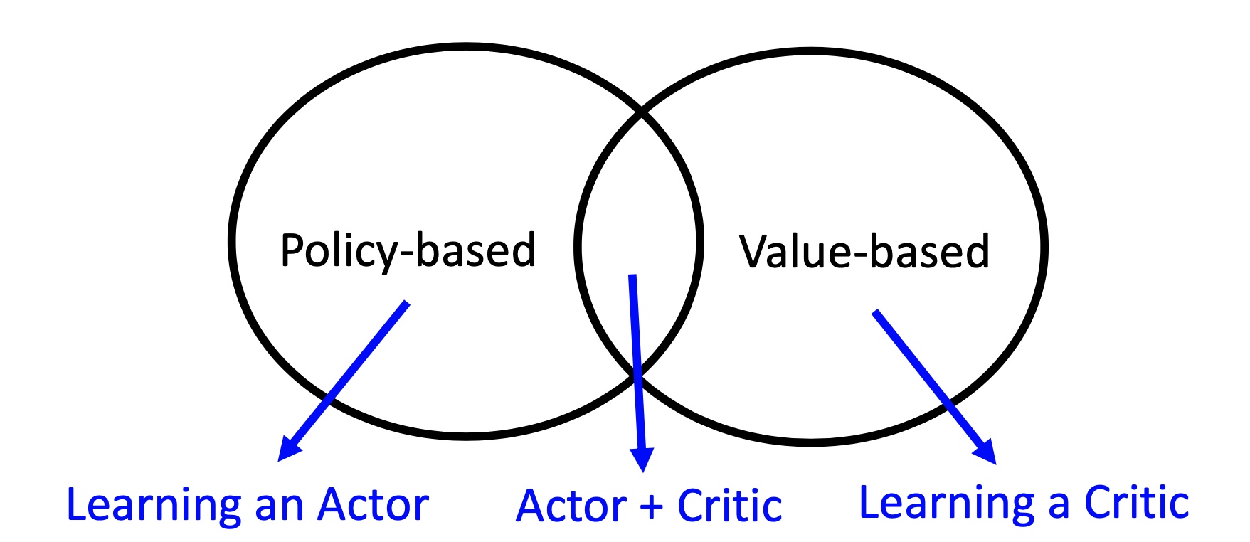
Q2: What do we mean by value-based， policy-based and collector-critic？ which algorithms can be classified as value-based，policy-based or actor-critic？what advantages do they have？what about the disadvantages？

• Answer：Value-based is to learn how to do critic (judging the value of an input state). Policy-based is to learn how to do actor (judging what action should be taken in an input state), and actor-critic is to learn decide critic while training the actor network. The relationship of these three classes can be well explained by the following diagram.

Q3: What are on-policy and off-policy？

• Answer：The on-policy algorithms are trained using the current policy. The policy used to generate sampled data is the same as the policy to be evaluated and improved. Off-policy algorithm, on the other hand, can be trained using the policy from the previous process, and the policy used to generate the sampled data is different from the policy to be evaluated and improved, i.e., the data generated is “off” the trajectory of the decision series determined by the policy to be optimised. On-policy and off-policy simply mean how training is done, and sometimes an algorithm may even have different ways of implementation of on-policy and off-policy.

Q4: What are online training and offline training？ How do we implement offline training？

• Answer： Offline training means the training uses fixed datasets as input instead of using a collector to interact with the environment. For example, behavioral cloning is a classic offline training algorithm. We usually input batch data in a fixed dataset, hence, offline RL is also called batch RL.

Q5: What are exploration and exploitation？What methods do we use to balance exploration and exploitation？

• Answer：Exploration is when an agent in RL is constantly exploring different states of the environment, while exploitation is when the agent selects the most rewarding action possible for the current state. There are many ways to balance exploration and exploitation. There are also different ways of implementation in different algorithms. With respect to sampling in discrete action spaces, one can follow a probability distribution or select randomly. With respect to sampling in continuous action spaces, one can follow a continuous distribution or add NOISE.

Q6: Why do we use replay buffer？ why do we need experience replay？

• Answer：By using the replay buffer, we can store the experiences in the buffer and sample the experiences in the buffer during subsequent training. Experience replay is a technique that saves samples from the system’s exploration of the environment and then samples them to update the model parameters.