A2C

Overview

A3C (Asynchronous advantage actor-critic) algorithm is a simple and lightweight framework for deep reinforcement learning that uses asynchronous gradient descent for optimization of deep neural network controllers. A2C(advantage actor-critic), on the other hand, is the synchronous version of A3C where where the policy gradient algorithm is combined with an advantage function to reduce variance.

Quick Facts

1. A2C is a model-free and policy-based RL algorithm.

2. A2C is an on-policy algorithm.

3. A2C supports both discrete and continuous action spaces.

4. A2C can be equipped with Recurrent Neural Network (RNN).

Key Equations or Key Graphs

A2C uses advantage estimation in the policy gradient. We implement the advantage by Generalized Advantage Estimation (GAE):

\[\nabla_{\theta} \log \pi\left(a_{t} \mid {s}_{t} ; \theta\right) \hat{A}^{\pi}\left(s_{t}, {a}_{t} ; \phi \right)\]

where the k-step advantage function is defined:

\[\sum_{i=0}^{k-1} \gamma^{i} r_{t+i}+\gamma^{k} \hat{V}^{\pi}\left(s_{t+k} ; \phi\right)-\hat{V}^{\pi}\left(s_{t} ; \phi\right)\]

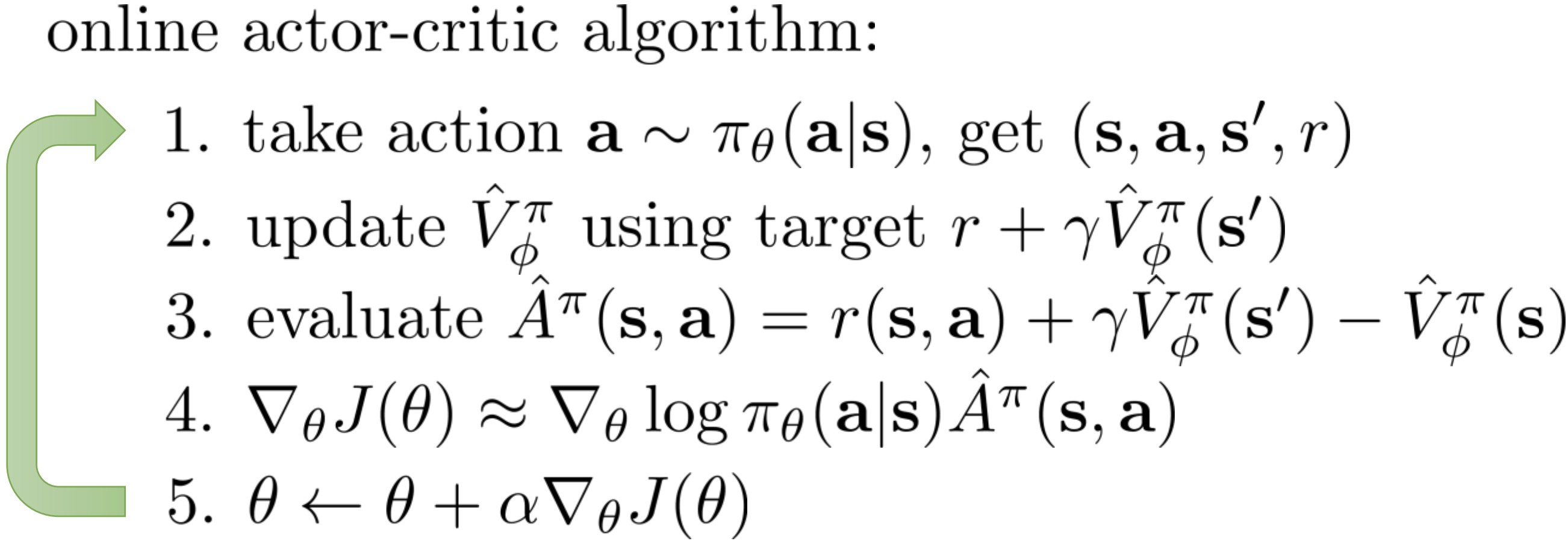
Pseudo-code

Note

Different from Q-learning, A2C(and other actor critic methods) alternates between policy estimation and policy improvement.

Extensions

A2C can be combined with:

• Multi-step learning

• RNN

• Generalized Advantage Estimation (GAE) GAE is proposed in High-Dimensional Continuous Control Using Generalized Advantage Estimation, it uses exponentially-weighted average of different steps of advantage estimators, to make trade-off between variance and bias of the estimation of the advantage:

  \[\hat{A}_{t}^{\mathrm{GAE}(\gamma, \lambda)}:=(1-\lambda)\left(\hat{A}_{t}^{(1)}+\lambda \hat{A}_{t}^{(2)}+\lambda^{2} \hat{A}_{t}^{(3)}+\ldots\right)\]

  where the k-step advantage estimator \(\hat{A}_t^{(k)}\) is defined as :

  \[\hat{A}_{t}^{(k)}:=\sum_{l=0}^{k-1} \gamma^{l} \delta_{t+l}^{V}=-V\left(s_{t}\right)+r_{t}+\gamma r_{t+1}+\cdots+\gamma^{k-1} r_{t+k-1}+\gamma^{k} V\left(s_{t+k}\right)\]

  When k=1, the estimator \(\hat{A}_t^{(1)}\) is the naive advantage estimator:

  \[\hat{A}_{t}^{(1)}:=\delta_{t}^{V} \quad=-V\left(s_{t}\right)+r_{t}+\gamma V\left(s_{t+1}\right)\]

  When GAE is used, the common values of \(\lambda\) usually belong to [0.8, 1.0].

Implementation

The default config is defined as follows:

class ding.policy.a2c.A2CPolicy(cfg: EasyDict, model: Module | None = None, enable_field: List[str] | None = None)

Overview:

Policy class of A2C (Advantage Actor-Critic) algorithm, proposed in https://arxiv.org/abs/1602.01783.

The network interface A2C used is defined as follows:

class ding.model.template.vac.VAC(obs_shape: int | SequenceType, action_shape: int | SequenceType | EasyDict, action_space: str = 'discrete', share_encoder: bool = True, encoder_hidden_size_list: SequenceType = [128, 128, 64], actor_head_hidden_size: int = 64, actor_head_layer_num: int = 1, critic_head_hidden_size: int = 64, critic_head_layer_num: int = 1, activation: Module | None = ReLU(), norm_type: str | None = None, sigma_type: str | None = 'independent', fixed_sigma_value: int | None = 0.3, bound_type: str | None = None, encoder: Module | None = None, impala_cnn_encoder: bool = False)

Overview:

The neural network and computation graph of algorithms related to (state) Value Actor-Critic (VAC), such as A2C/PPO/IMPALA. This model now supports discrete, continuous and hybrid action space. The VAC is composed of four parts: actor_encoder, critic_encoder, actor_head and critic_head. Encoders are used to extract the feature from various observation. Heads are used to predict corresponding value or action logit. In high-dimensional observation space like 2D image, we often use a shared encoder for both actor_encoder and critic_encoder. In low-dimensional observation space like 1D vector, we often use different encoders.

Interfaces:

__init__, forward, compute_actor, compute_critic, compute_actor_critic.

compute_actor(x: Tensor) → Dict

Overview:

VAC forward computation graph for actor part, input observation tensor to predict action logit.

Arguments:

• x (torch.Tensor): The input observation tensor data.

Returns:

• outputs (Dict): The output dict of VAC’s forward computation graph for actor, including logit.

ReturnsKeys:

• logit (torch.Tensor): The predicted action logit tensor, for discrete action space, it will be the same dimension real-value ranged tensor of possible action choices, and for continuous action space, it will be the mu and sigma of the Gaussian distribution, and the number of mu and sigma is the same as the number of continuous actions. Hybrid action space is a kind of combination of discrete and continuous action space, so the logit will be a dict with action_type and action_args.

Shapes:

• logit (torch.Tensor): \((B, N)\), where B is batch size and N is action_shape

Examples:

>>> model = VAC(64, 64)
>>> inputs = torch.randn(4, 64)
>>> actor_outputs = model(inputs,'compute_actor')
>>> assert actor_outputs['logit'].shape == torch.Size([4, 64])

compute_actor_critic(x: Tensor) → Dict

Overview:

VAC forward computation graph for both actor and critic part, input observation tensor to predict action logit and state value.

Arguments:

• x (torch.Tensor): The input observation tensor data.

Returns:

• outputs (Dict): The output dict of VAC’s forward computation graph for both actor and critic, including logit and value.

ReturnsKeys:

• logit (torch.Tensor): The predicted action logit tensor, for discrete action space, it will be the same dimension real-value ranged tensor of possible action choices, and for continuous action space, it will be the mu and sigma of the Gaussian distribution, and the number of mu and sigma is the same as the number of continuous actions. Hybrid action space is a kind of combination of discrete and continuous action space, so the logit will be a dict with action_type and action_args.

• value (torch.Tensor): The predicted state value tensor.

Shapes:

• logit (torch.Tensor): \((B, N)\), where B is batch size and N is action_shape

• value (torch.Tensor): \((B, )\), where B is batch size, (B, 1) is squeezed to (B, ).

Examples:

>>> model = VAC(64, 64)
>>> inputs = torch.randn(4, 64)
>>> outputs = model(inputs,'compute_actor_critic')
>>> assert critic_outputs['value'].shape == torch.Size([4])
>>> assert outputs['logit'].shape == torch.Size([4, 64])

Note

compute_actor_critic interface aims to save computation when shares encoder and return the combination dict output.

compute_critic(x: Tensor) → Dict

Overview:

VAC forward computation graph for critic part, input observation tensor to predict state value.

Arguments:

• x (torch.Tensor): The input observation tensor data.

Returns:

• outputs (Dict): The output dict of VAC’s forward computation graph for critic, including value.

ReturnsKeys:

• value (torch.Tensor): The predicted state value tensor.

Shapes:

• value (torch.Tensor): \((B, )\), where B is batch size, (B, 1) is squeezed to (B, ).

Examples:

>>> model = VAC(64, 64)
>>> inputs = torch.randn(4, 64)
>>> critic_outputs = model(inputs,'compute_critic')
>>> assert critic_outputs['value'].shape == torch.Size([4])

forward(x: Tensor, mode: str) → Dict

Overview:

VAC forward computation graph, input observation tensor to predict state value or action logit. Different mode will forward with different network modules to get different outputs and save computation.

Arguments:

• x (torch.Tensor): The input observation tensor data.

• mode (str): The forward mode, all the modes are defined in the beginning of this class.

Returns:

• outputs (Dict): The output dict of VAC’s forward computation graph, whose key-values vary from different mode.

Examples (Actor):

>>> model = VAC(64, 128)
>>> inputs = torch.randn(4, 64)
>>> actor_outputs = model(inputs,'compute_actor')
>>> assert actor_outputs['logit'].shape == torch.Size([4, 128])

Examples (Critic):

>>> model = VAC(64, 64)
>>> inputs = torch.randn(4, 64)
>>> critic_outputs = model(inputs,'compute_critic')
>>> assert actor_outputs['logit'].shape == torch.Size([4, 64])

Examples (Actor-Critic):

>>> model = VAC(64, 64)
>>> inputs = torch.randn(4, 64)
>>> outputs = model(inputs,'compute_actor_critic')
>>> assert critic_outputs['value'].shape == torch.Size([4])
>>> assert outputs['logit'].shape == torch.Size([4, 64])

The policy gradient and value update of A2C is implemented as follows:

def a2c_error(data: namedtuple) -> namedtuple:
    logit, action, value, adv, return_, weight = data
    if weight is None:
        weight = torch.ones_like(value)
    dist = torch.distributions.categorical.Categorical(logits=logit)
    logp = dist.log_prob(action)
    entropy_loss = (dist.entropy() * weight).mean()
    policy_loss = -(logp * adv * weight).mean()
    value_loss = (F.mse_loss(return_, value, reduction='none') * weight).mean()
    return a2c_loss(policy_loss, value_loss, entropy_loss)

Note

we apply GAE to calculate the advantage when update the actor network with the GAE default parameter gae_lambda =0.95. The target for the update for the value network is obtained by the value function at the current time step plus the advantage function calculated in collectors.

Benchmark

environment	best mean reward	evaluation results	config link	comparison
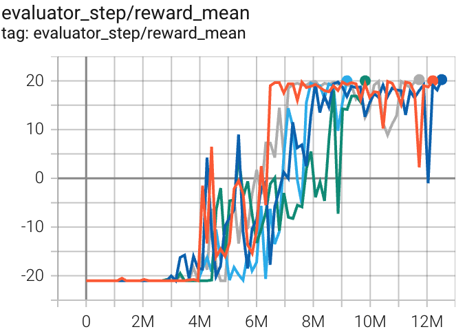
Pong (PongNoFrameskip-v4)	20		config_link_p	Sb3(17)
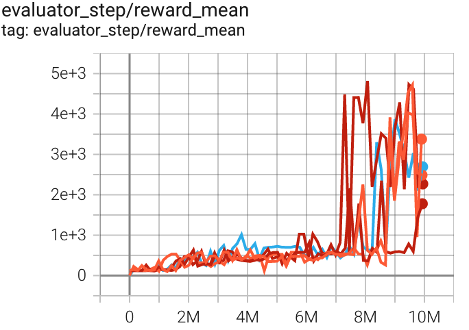
Qbert (QbertNoFrameskip-v4)	4819		config_link_q	Sb3(3882) Rllib(3620)
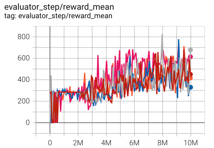
SpaceInvaders (SpaceInvadersNoFrame skip-v4)	826		config_link_s	Sb3(627) Rllib(692)

P.S.：

1. The above results are obtained by running the same configuration on five different random seeds (0, 1, 2, 3, 4)

References

Volodymyr Mnih, Adrià Puigdomènech Badia, Mehdi Mirza, Alex Graves, Timothy P. Lillicrap, Tim Harley, David Silver, Koray Kavukcuoglu: “Asynchronous Methods for Deep Reinforcement Learning”, 2016, ICML 2016; arXiv:1602.01783. https://arxiv.org/abs/1602.01783

Other Public Implementations

• Baselines

• sb3

• rllib (Ray)

• tianshou