FQF
Overview
FQF was proposed in Fully Parameterized Quantile Function for Distributional Reinforcement Learning. The key difference between FQF and IQN is that FQF additionally introduces the fraction proposal network, a parametric function trained to generate tau in [0, 1], while IQN samples tau from a base distribution, e.g. U([0, 1]).
Quick Facts
FQF is a model-free and value-based distibutional RL algorithm.
FQF only support discrete action spaces.
FQF is an off-policy algorithm.
Usually, FQF use eps-greedy or multinomial sample for exploration.
FQF can be equipped with RNN.
Key Equations or Key Graphs
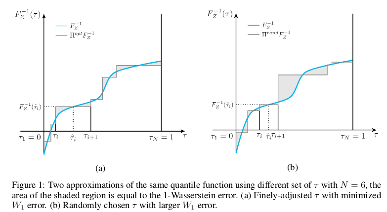
For any continuous quantile function \(F_{Z}^{-1}\) that is non-decreasing, define the 1-Wasserstein loss of \(F_{Z}^{-1}\) and \(F_{Z}^{-1, \tau}\) by
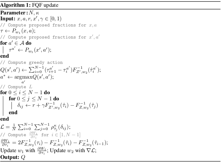
Note that as \(W_{1}\) is not computed, we can’t directly perform gradient descent for the fraction proposal network. Instead, we assign \(\frac{\partial W_{1}}{\partial \tau_{i}}\) to the optimizer.
\(\frac{\partial W_{1}}{\partial \tau_{i}}\) is given by
Like implicit quantile networks, a learned quantile tau is encoded into an embedding vector via:
Then the quantile embedding is element-wise multiplied by the embedding of the observation of the environment, and the subsequent fully-connected layers map the resulted product vector to the respective quantile value.
The advantage of FQF over IQN can be showed in this picture:
Pseudo-code
Extensions
FQF can be combined with:
PER (Prioritized Experience Replay)
Tip
Whether PER improves FQF depends on the task and the training strategy.
Multi-step TD-loss
Double (target) Network
RNN
Implementation
Tip
Our benchmark result of FQF uses the same hyper-parameters as DQN except the FQF’s exclusive hyper-parameter, the number of quantiles, which is empirically set as 32. Intuitively, the advantage of trained quantile fractions compared to random ones will be more observable at smaller N. At larger N when both trained quantile fractions and random ones are densely distributed over [0, 1], the differences between FQF and IQN becomes negligible.
The default config of FQF is defined as follows:
- class ding.policy.fqf.FQFPolicy(cfg: EasyDict, model: Module | None = None, enable_field: List[str] | None = None)[source]
- Overview:
Policy class of FQF (Fully Parameterized Quantile Function) algorithm, proposed in https://arxiv.org/pdf/1911.02140.pdf.
- Config:
ID
Symbol
Type
Default Value
Description
Other(Shape)
1
typestr
fqf
RL policy register name, refer toregistryPOLICY_REGISTRYthis arg is optional,a placeholder2
cudabool
False
Whether to use cuda for networkthis arg can be diff-erent from modes3
on_policybool
False
Whether the RL algorithm is on-policyor off-policy4
prioritybool
True
Whether use priority(PER)priority sample,update priority6
other.eps.startfloat
0.05
Start value for epsilon decay. It’ssmall because rainbow use noisy net.7
other.eps.endfloat
0.05
End value for epsilon decay.8
discount_factorfloat
0.97, [0.95, 0.999]
Reward’s future discount factor, aka.gammamay be 1 when sparsereward env9
nstepint
3, [3, 5]
N-step reward discount sum for targetq_value estimation10
learn.updateper_collectint
3
How many updates(iterations) to trainafter collector’s one collection. Onlyvalid in serial trainingthis args can be varyfrom envs. Bigger valmeans more off-policy11
learn.kappafloat
/
Threshold of Huber loss
The network interface FQF used is defined as follows:
- class ding.model.template.q_learning.FQF(obs_shape: int | SequenceType, action_shape: int | SequenceType, encoder_hidden_size_list: SequenceType = [128, 128, 64], head_hidden_size: int | None = None, head_layer_num: int = 1, num_quantiles: int = 32, quantile_embedding_size: int = 128, activation: Module | None = ReLU(), norm_type: str | None = None)[source]
- Overview:
The neural network structure and computation graph of FQF, which combines distributional RL and DQN. You can refer to paper Fully Parameterized Quantile Function for Distributional Reinforcement Learning https://arxiv.org/pdf/1911.02140.pdf for more details.
- Interface:
__init__,forward
- forward(x: Tensor) Dict[source]
- Overview:
Use encoded embedding tensor to predict FQF’s output. Parameter updates with FQF’s MLPs forward setup.
- Arguments:
- x (
torch.Tensor): The encoded embedding tensor with
(B, N=hidden_size).
- x (
- Returns:
outputs (
Dict): Dict containing keywordslogit(torch.Tensor),q(torch.Tensor),quantiles(torch.Tensor),quantiles_hats(torch.Tensor),q_tau_i(torch.Tensor),entropies(torch.Tensor).
- Shapes:
x: \((B, N)\), where B is batch size and N is head_hidden_size.
logit: \((B, M)\), where M is action_shape.
q: \((B, num_quantiles, M)\).
quantiles: \((B, num_quantiles + 1)\).
quantiles_hats: \((B, num_quantiles)\).
q_tau_i: \((B, num_quantiles - 1, M)\).
entropies: \((B, 1)\).
- Examples:
>>> model = FQF(64, 64) # arguments: 'obs_shape' and 'action_shape'
>>> inputs = torch.randn(4, 64)
>>> outputs = model(inputs)
>>> assert isinstance(outputs, dict)
>>> assert outputs['logit'].shape == torch.Size([4, 64])
>>> # default num_quantiles: int = 32
>>> assert outputs['q'].shape == torch.Size([4, 32, 64])
>>> assert outputs['quantiles'].shape == torch.Size([4, 33])
>>> assert outputs['quantiles_hats'].shape == torch.Size([4, 32])
>>> assert outputs['q_tau_i'].shape == torch.Size([4, 31, 64])
>>> assert outputs['quantiles'].shape == torch.Size([4, 1])
The bellman updates of FQF used is defined in the function fqf_nstep_td_error of ding/rl_utils/td.py.
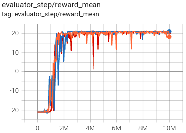
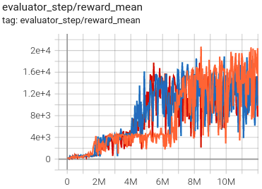
Benchmark
environment |
best mean reward |
evaluation results |
config link |
comparison |
|---|---|---|---|---|
Pong (PongNoFrameskip-v4) |
21 |
|
Tianshou(20.7) |
|
Qbert (QbertNoFrameskip-v4) |
23416 |
|
Tianshou(16172.5) |
|
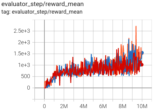
SpaceInvaders (SpaceInvadersNoFrame skip-v4) |
2727.5 |
|
Tianshou(2482) |
- P.S.:
The above results are obtained by running the same configuration on three different random seeds (0, 1, 2).
References
(FQF) Derek Yang, Li Zhao, Zichuan Lin, Tao Qin, Jiang Bian, Tieyan Liu: “Fully Parameterized Quantile Function for Distributional Reinforcement Learning”, 2019; arXiv:1911.02140. https://arxiv.org/pdf/1911.02140