ICM¶

Overview¶

ICM (Intrinsic Curiosity Module) was first proposed in the paper Curiosity-driven Exploration by Self-supervised Prediction, It is used to study how to let the agent explore more unexperienced states and learn skills in a sparse reward environment. Its main idea is to use ‘curiosity’ as a signal of intrinsic reward, allowing the agent to explore the environment more efficiently.

The difficulties the algorithm trying to solve:

High-dimensional continuous state space (such as image information) is difficult to establish an intuitive dynamic model, ie \(p_\theta(s_{t+1}, a_t)\) ;
The correlation between the observation in the environment and the agent’s own behavior is different, which can be roughly divided into:
1. Elements that the agent can directly control (such as the position and speed of the vehicle in the autonomous driving scene);
2. Elements which are not controlled by the agent, but will affect the agent (such as the position and speed of his car in the automatic driving scene);
3. Elements that are neither controlled by the agent nor affect the agent (such as the intensity of sunlight in an autonomous driving scene, although it will affect the sensor, it will not affect the driving behavior in essence).

For the above three types of observation elements, we want to extract the environmental features in (a) and (b) two contexts, (these two environmental features are related to the action of the agent), while ignoring (c) the contextual features (this This kind of environment feature has nothing to do with the action of the agent).

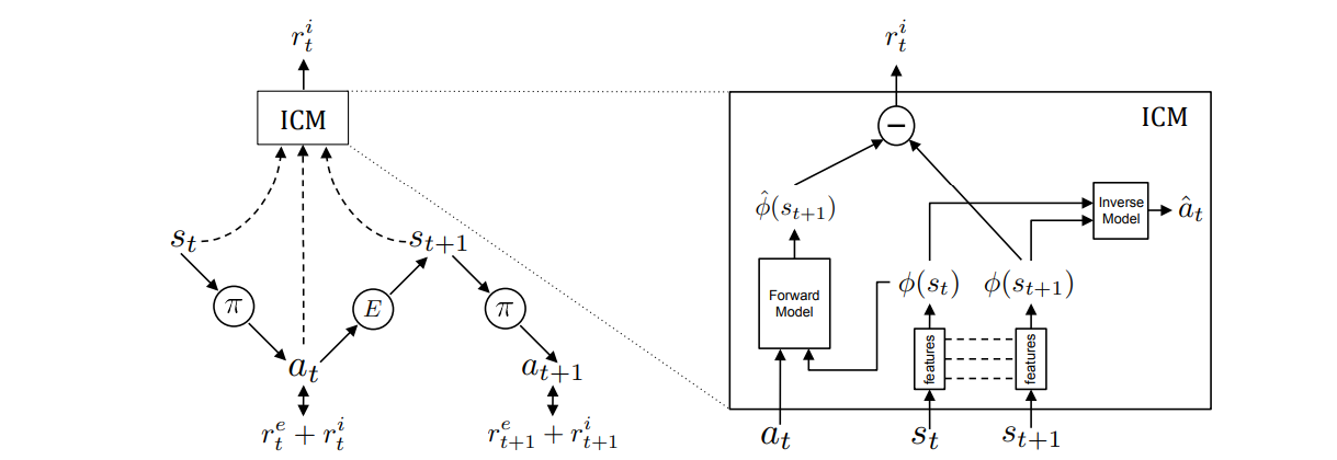
Features: Description of feature space Use a feature space to represent the environment, instead of directly using the original observation to represent the environment, so that features only related to agent actions can be extracted, and features unrelated to environmental features can be ignored. . Based on the representation of this feature space, a reward module and a forward model are proposed. Reward model The core idea is to estimate the action value adopted by the current state through the representation of the current state and the state at the next moment. The more accurate the estimation of the current action, the better the representation of the environmental elements that the agent can control. Forward model The core idea is to estimate the state representation of the next moment through the current state representation and the current action. This model can make the learned state representations more predictable.

The agent of ICM has two subsystems: one is the intrinsic reward generator, which takes the prediction error of the forward model as the intrinsic reward (so the total reward is the sum of the intrinsic reward and the sparse environment reward); the other The subsystem is a policy network that outputs a sequence of actions. The optimization goal of training the policy network is the expectation of the total score, so the optimization of the policy will not only consider getting more rewards from the sparse environment, but also explore actions that have not been seen before in order to get more intrinsic rewards.

Quick Facts¶

The baseline reinforcement learning algorithm of ICM is A3C , you can refer to our implementation A2C , if you want to implement A3C, you can use multiple environments to train at the same time.
In the follow-up work Large-Scale Study of Curiosity-Driven Learning, the baseline algorithm used is PPO, you can refer to our implementation PPO, through the PPO algorithm, only a small amount of hyperparameter fine-tuning is required to obtain a robust learning effect .
Although both the reward model and the forward model will participate in the calculation of loss, only the forward model will be used as an intrinsic reward. The larger the loss of the forward model, the more inaccurate the estimation of the state characteristics at the next moment based on the current state characteristics and the current action, that is, this state has not been encountered before, and it is worth exploring; the reward model is not an intrinsic reward, its role is mainly to better help characterize the environmental features related to agent actions in the process of feature space extraction.
Reward normalization. Since the reward is unstable, it is necessary to normalize the reward to [0, 1] to make the learning more stable. Here we use the maximum and minimum normalization method.
Feature normalization. By integrating intrinsic and extrinsic rewards, it is important to ensure that intrinsic rewards scale across different feature representations, which can be achieved through batch normalization.
More actors (more collectors in DI-engine): Adding more parallel actors can make training more stable.

Key Equations or Key Graphs¶

The overall training and calculation process of the ICM algorithm is as follows:

1. As shown in the figure on the left, the agent samples the action a in the state \(s_t\) through the current policy \(\pi\) and executes it, and finally obtains the state \(s_{t+1}\). The total reward is the sum of two partial rewards, one part is the external reward \(r_t^e\), that is, the sparse reward obtained in the environment; the other part is the intrinsic reward obtained by the ICM \(r_t^ｉ\) (The specific calculation process is given in step 4), the final strategy needs to achieve the purpose of training by optimizing the total reward. The specific formula is as follows:

\(r_t=r_t^i + r_t^e\)

\({\max}_{\theta_p}\mathbb{E}_{\pi(s_t;\theta_p)}[\Sigma_t r_t]\)

In the reward module of ICM, it first extracts the eigenvectors after characterization by \(s_t\) and \(s_{t+1}\),:math:Phi(s_t; theta_E) and \(\Phi(s_{t+1}; \theta_E)\) as input (reduce them to \(\Phi(s_t)\) and \(\Phi(s_{t+1 })\)), and output the predicted action value \(a_t\)

\(\hat{a_t}=g(\Phi(s_t),\Phi(s_{t+1}) ; \theta_I)\)

\({\min}_{\theta_I, \theta_E} L_i(\hat{a_t},a_t)\)

Here \(\hat{a_t}\) is the predicted value of \(a_t\) and \(L_I\) describes the difference between the two (cross entropy loss). The smaller the difference, the more accurate the estimation of the current action, and the better the representation of the environmental elements that the agent can control.

3. The forward model of ICM will take \(\Phi(s_t)\) and action value　\(a_t\) as input, and output the predicted value of the feature vector of the state at the next moment:math:hat{Phi}(s_{t+1}) The error between the predicted feature vector at the next moment and the real feature vector is used as the intrinsic reward.

\(\hat{\phi(s_{t+1})}=f(\Phi(s_t),a_t) ; \theta_F)\)

\({\min}_{\theta_F, \theta_E} L_F(\hat{\phi(s_{t+1})},\phi(s_{t+1}))\)

Here, \(L_F\) describes the difference between \(\hat{\phi(s_{t+1})}\) and \(\phi(s_{t+1})\) (L2 loss), through the learning of the forward model, the learned feature representation can be more predictable.

The intrinsic reward can be characterized by the difference between \(\hat{\phi(s_{t+1})}\) and \(\phi(s_{t+1})\):

\(r_i^t = \frac{\eta}{2} (\| \hat{\phi(s_{t+1})} - \phi(s_{t+1}) \|)_2^ 2\)

Summarize: Through the forward model and the reward model, ICM will extract more features of environmental elements that will be affected by the agent; for those environmental elements (such as noise) that cannot be affected by the agent’s actions, there will be no intrinsic reward, thus improving the exploration strategy in robustness. At the same time, 1-4 can also be written as an optimization function:

\({\min}_{\theta_P,\theta_I,\theta_F,\theta_E} [- \lambda \mathbb{E}_{\pi(s_t;\theta_p)}[\Sigma_t r_t] + (1 -\beta)L_I + \beta LF]\)

Here: math:beta in [0,1] is used to weigh the weight of forward model error and reward model error; \(\lambda >0\) is used to characterize the importance of policy gradient error to the intrinsic signal degree.

Important Implementation Details¶

1. Reward normalization. Since the agent is in different stages and environments, the magnitude of the reward may change drastically. If it is directly used for subsequent calculations, it is easy to cause instability in subsequent learning. In our implementation, it is normalized to [0, 1] according to the following maximum and minimum normalization formula:

reward = (reward - reward.min()) / (reward.max() - reward.min() + 1e-8)

2. Use a residual network to fit the forward model. Since the representation dimension of observation is relatively large, the action value is often a discrete value. Therefore, when calculating the forward model, the residual network can better retain the information of the action value, so as to obtain a better environmental representation.

pred_next_state_feature_orig = torch.cat((encode_state, action), 1)
pred_next_state_feature_orig = self.forward_net_1(pred_next_state_feature_orig)
for i in range(4):
    pred_next_state_feature = self.residual[i * 2](torch.cat((pred_next_state_feature_orig, action), 1))
    pred_next_state_feature_orig = self.residual[i * 2 + 1](torch.cat((pred_next_state_feature, action), 1)
    ) + pred_next_state_feature_orig
pred_next_state_feature = self.forward_net_2(torch.cat((pred_next_state_feature_orig, action), 1))

Implementations¶

The interface for the Intrinsic Curiosity Model ( ICMRewardModel ) is defined as follows:

class ding.reward_model.icm_reward_model.ICMRewardModel(config: EasyDict, device: str, tb_logger: SummaryWriter)[source]

Overview:

The ICM reward model class (https://arxiv.org/pdf/1705.05363.pdf)

Interface:

estimate, train, collect_data, clear_data, __init__, _train, load_state_dict, state_dict

Config:

ID	Symbol	Type	Default Value	Description	Other(Shape)
1	`type`	str	icm	Reward model register name, refer to registry `REWARD_MODEL_REGISTRY`
2	`intrinsic_` `reward_type`	str	add	the intrinsic reward type	including add, new , or assign
3	`learning_rate`	float	0.001	The step size of gradient descent
4	`obs_shape`	Tuple( [int, list])	6	the observation shape
5	`action_shape`	int	7	the action space shape
6	`batch_size`	int	64	Training batch size
7	`hidden` `_size_list`	list (int)	[64, 64, 128]	the MLP layer shape
8	`update_per_` `collect`	int	100	Number of updates per collect
9	`reverse_scale`	float	1	the importance weight of the forward and reverse loss
10	`intrinsic_` `reward_weight`	float	0.003	the weight of intrinsic reward	r = w*r_i + r_e
11	`extrinsic_` `reward_norm`	bool	True	Whether to normlize extrinsic reward
12	`extrinsic_` `reward_norm_max`	int	1	the upper bound of the reward normalization
13	`clear_buffer` `_per_iters`	int	1	clear buffer per fixed iters	make sure replay buffer’s data count isn’t too few. (code work in entry)

clear_data() → None[source]

Overview:: Clearing training data. This can be a side effect function which clears the data attribute in self

collect_data(data: list) → None[source]

Overview:

Collecting training data in designated formate or with designated transition.

Arguments:

data (Any): Raw training data (e.g. some form of states, actions, obs, etc)

Returns / Effects:

This can be a side effect function which updates the data attribute in self

estimate(data: list) → List[Dict][source]

Overview:

estimate reward

Arguments:

data (List): the list of data used for estimation

Returns / Effects:

This can be a side effect function which updates the reward value
If this function returns, an example returned object can be reward (Any): the estimated reward

train() → None[source]

Overview:

Training the reward model

Arguments:

data (Any): Data used for training

Effects:

This is mostly a side effect function which updates the reward model

ICMNetwork¶

First we define the class ICMNetwork which involves four kinds of neural networks:

self.feature: extract the features of observation;

self.inverse_net: The inverse model of the ICM network, which outputs a predicted action by taking two successive frames of feature features as input

self.residual: Participate in the forward model of the ICM network, and make the features more obvious by concat the output of the action and the intermediate layer for many times

self.forward_net: Participate in the forward model of the ICM network, responsible for outputting the feature at the moment of \(s_{t+1}\)

class ICMNetwork(nn.Module):
r"""
Intrinsic Curiosity Model (ICM Module)
Implementation of:
[1] Curiosity-driven Exploration by Self-supervised Prediction
Pathak, Agrawal, Efros, and Darrell - UC Berkeley - ICML 2017.
https://arxiv.org/pdf/1705.05363.pdf
[2] Code implementation reference:
https://github.com/pathak22/noreward-rl
https://github.com/jcwleo/curiosity-driven-exploration-pytorch

1) Embedding observations into a latent space
2) Predicting the action logit given two consecutive embedded observations
3) Predicting the next embedded obs, given the embedded former observation and action
"""

def __init__(self, obs_shape: Union[int, SequenceType], hidden_size_list: SequenceType, action_shape: int) -> None:
    super(ICMNetwork, self).__init__()
    if isinstance(obs_shape, int) or len(obs_shape) == 1:
        self.feature = FCEncoder(obs_shape, hidden_size_list)
    elif len(obs_shape) == 3:
        self.feature = ConvEncoder(obs_shape, hidden_size_list)
    else:
        raise KeyError(
            "not support obs_shape for pre-defined encoder: {}, please customize your own ICM model".
            format(obs_shape)
        )
    self.action_shape = action_shape
    feature_output = hidden_size_list[-1]
    self.inverse_net = nn.Sequential(nn.Linear(feature_output * 2, 512), nn.ReLU(), nn.Linear(512, action_shape))
    self.residual = nn.ModuleList(
        [
            nn.Sequential(
                nn.Linear(action_shape + 512, 512),
                nn.LeakyReLU(),
                nn.Linear(512, 512),
            ) for _ in range(8)
        ]
    )
    self.forward_net_1 = nn.Sequential(nn.Linear(action_shape + feature_output, 512), nn.LeakyReLU())
    self.forward_net_2 = nn.Linear(action_shape + 512, feature_output)

def forward(self, state: torch.Tensor, next_state: torch.Tensor,
            action_long: torch.Tensor) -> Tuple[torch.Tensor, torch.Tensor, torch.Tensor]:
    r"""
    Overview:
        Use observation, next_observation and action to genearte ICM module
        Parameter updates with ICMNetwork forward setup.
    Arguments:
        - state (:obj:`torch.Tensor`):
            The current state batch
        - next_state (:obj:`torch.Tensor`):
            The next state batch
        - action_long (:obj:`torch.Tensor`):
            The action batch
    Returns:
        - real_next_state_feature (:obj:`torch.Tensor`):
            Run with the encoder. Return the real next_state's embedded feature.
        - pred_next_state_feature (:obj:`torch.Tensor`):
            Run with the encoder and residual network. Return the predicted next_state's embedded feature.
        - pred_action_logit (:obj:`torch.Tensor`):
            Run with the encoder. Return the predicted action logit.
    Shapes:
        - state (:obj:`torch.Tensor`): :math:`(B, N)`, where B is the batch size and N is ''obs_shape''
        - next_state (:obj:`torch.Tensor`): :math:`(B, N)`, where B is the batch size and N is ''obs_shape''
        - action_long (:obj:`torch.Tensor`): :math:`(B)`, where B is the batch size''
        - real_next_state_feature (:obj:`torch.Tensor`): :math:`(B, M)`, where B is the batch size
        and M is embedded feature size
        - pred_next_state_feature (:obj:`torch.Tensor`): :math:`(B, M)`, where B is the batch size
        and M is embedded feature size
        - pred_action_logit (:obj:`torch.Tensor`): :math:`(B, A)`, where B is the batch size
        and A is the ''action_shape''
    """
    action = one_hot(action_long, num=self.action_shape)
    encode_state = self.feature(state)
    encode_next_state = self.feature(next_state)
    # get pred action logit
    concat_state = torch.cat((encode_state, encode_next_state), 1)
    pred_action_logit = self.inverse_net(concat_state)
    # ---------------------

    # get pred next state
    pred_next_state_feature_orig = torch.cat((encode_state, action), 1)
    pred_next_state_feature_orig = self.forward_net_1(pred_next_state_feature_orig)

    # residual
    for i in range(4):
        pred_next_state_feature = self.residual[i * 2](torch.cat((pred_next_state_feature_orig, action), 1))
        pred_next_state_feature_orig = self.residual[i * 2 + 1](
            torch.cat((pred_next_state_feature, action), 1)
        ) + pred_next_state_feature_orig
    pred_next_state_feature = self.forward_net_2(torch.cat((pred_next_state_feature_orig, action), 1))
    real_next_state_feature = encode_next_state
    return real_next_state_feature, pred_next_state_feature, pred_action_logit

Results¶

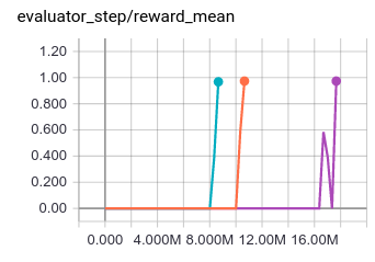
Environment: MiniGrid-DoorKey-8x8-v0; Baseline algorithm: ppo_offpolicy, The three lines of the experiment are three seeds, the ids are: 0, 10, 20

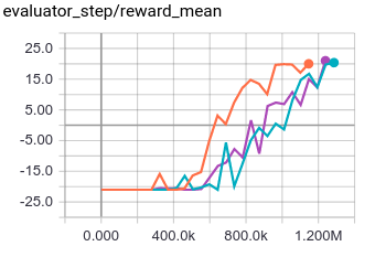
Environment: PongNoFrameskip-v4; Baseline algorithm: ppo_offpolicy, The three lines of the experiment are three seeds, the ids are: 0, 10, 20

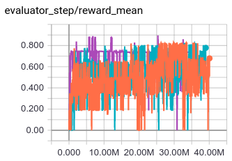
Environment: MiniGrid-FourRooms-v0; Baseline algorithm: ppo_offpolicy, The three lines of the experiment are three seeds, the ids are: 0, 10, 20

References¶

Pathak D, Agrawal P, Efros A A, et al. Curiosity-driven exploration by self-supervised prediction[C]//International conference on machine learning. PMLR, 2017: 2778-2787.
Burda Y, Edwards H, Storkey A, et al. Exploration by random network distillation[J]. https://arxiv.org/abs/1810.12894v1. arXiv:1810.12894, 2018.