CLI Usage
From treevalue version 0.1.0, simple CLI (Command Line Interface) is provided to simplify some operations and optimize the use experience. This page will introduce the usage of cli.
Version Display
You can see the version information with the following command typing into the terminal:
1 | treevalue -v
|
The output should be
1 2 | Treevalue, version 1.5.0. Developed by HansBug (hansbug@buaa.edu.cn), DI-engine's Contributors. |
Note
You can check if the treevalue package is installed properly with this command line since version 0.1.0.
Help Information Display
You can see the help information of this cli by the following command line:
1 | treevalue -h
|
The output should be
1 2 3 4 5 6 7 8 9 | Usage: treevalue [OPTIONS] COMMAND [ARGS]... Options: -v, --version Show package's version information. -h, --help Show this message and exit. Commands: export Export trees to binary files, compression is available. graph Generate graph by trees and graphviz elements. |
There are several sub commands in treevalue cli, and they will be introduced in the following sections.
Exporting Trees to Binary
First, let’s see what is in treevalue export sub command.
1 2 3 4 5 6 7 8 9 10 11 12 13 14 | Usage: treevalue export [OPTIONS]
Export trees to binary files, compression is available.
Options:
-t, --tree TEXT Trees to be imported from packages, such as '-t
my_tree.t1'.
-o, --output FILE Output file path, multiple output is supported.
-d, --directory DIRECTORY Directory to save the exported trees.
-c, --compress TEXT Compress algorithm, can be a single lib name or a
tuple, default use 'zlib'.
-r, --raw Disable all the compression, just export the raw
data.
-h, --help Show this message and exit.
|
In this sub command, we can export a tree value object to binary file with dump, dumps function define in module treevalue.tree.tree.
Note
For further information, take a look at:
Export One Tree
Before exporting, we prepare a python source code file tree_demo.py with the content of
1 2 3 4 5 | from treevalue import FastTreeValue t1 = FastTreeValue({'a': 1, 'b': 2, 'x': {'c': 3, 'd': 4}}) t2 = FastTreeValue({'a': 11, 'b': 24, 'x': {'c': 30, 'd': 47}}) t3 = t1 + t2 |
And then we can to export t1 to binary file, like this
1 2 | treevalue export -t 'tree_demo.t1' -o export_t1.dat.btv ls -al export_t1.dat.btv |
A binary file named export_t1.dat.btv will be exported.
1 2 | Exporting tree 't1.btv' to binary file '/tmp/tmp4q2ykbbk/695148caffa69afacf344700cfd634bb66038ba6/docs/source/tutorials/cli_usage/export_t1.dat.btv' ... OK. -rw-r--r-- 1 runner docker 156 Oct 16 13:40 export_t1.dat.btv |
The binary file is exported with the dump function, and the compression algorithm used is the default one zlib.
Export Multiple Trees Once
We can export multiple trees at one time with the following command
1 2 | treevalue export -t 'tree_demo.*' -o 'me_t1.dat.btv' -o 'me_t2.dat.btv' -o 'me_t3.dat.btv' ls -al me_*.btv |
Three binary files named me_t1.dat.btv, me_t2.dat.btv and me_t3.dat.btv will be exported.
1 2 3 4 5 6 | Exporting tree 't1.btv' to binary file '/tmp/tmp4q2ykbbk/695148caffa69afacf344700cfd634bb66038ba6/docs/source/tutorials/cli_usage/me_t1.dat.btv' ... OK. Exporting tree 't2.btv' to binary file '/tmp/tmp4q2ykbbk/695148caffa69afacf344700cfd634bb66038ba6/docs/source/tutorials/cli_usage/me_t2.dat.btv' ... OK. Exporting tree 't3.btv' to binary file '/tmp/tmp4q2ykbbk/695148caffa69afacf344700cfd634bb66038ba6/docs/source/tutorials/cli_usage/me_t3.dat.btv' ... OK. -rw-r--r-- 1 runner docker 156 Oct 16 13:40 me_t1.dat.btv -rw-r--r-- 1 runner docker 156 Oct 16 13:40 me_t2.dat.btv -rw-r--r-- 1 runner docker 155 Oct 16 13:40 me_t3.dat.btv |
Export Tree with Compression
We can assign compression algorithm by the -c option, like this
1 2 | treevalue export -t 'tree_demo.t1' -c gzip -o compress_t1.dat.btv ls -al compress_t1.dat.btv |
The binary file named compress_t1.dat.btv will be exported with the gzip compression, and will be able to be loaded with treevalue graph cli and load function without the assignment of decompression algorithm.
1 2 | Exporting tree 't1.btv' to binary file '/tmp/tmp4q2ykbbk/695148caffa69afacf344700cfd634bb66038ba6/docs/source/tutorials/cli_usage/compress_t1.dat.btv' ... OK. -rw-r--r-- 1 runner docker 168 Oct 16 13:40 compress_t1.dat.btv |
I DO NOT NEED COMPRESSION
If you do not need compression due to the reasons like the time scarcity, you can easily disable the compression.
1 2 | treevalue export -t 'tree_demo.t1' -r -o raw_t1.dat.btv ls -al raw_t1.dat.btv |
The dumped binary file raw_t1.dat.btv will not be compressed due to the -r option.
1 2 | Exporting tree 't1.btv' to binary file '/tmp/tmp4q2ykbbk/695148caffa69afacf344700cfd634bb66038ba6/docs/source/tutorials/cli_usage/raw_t1.dat.btv' ... OK. -rw-r--r-- 1 runner docker 145 Oct 16 13:40 raw_t1.dat.btv |
Note
You may feel puzzled that why the size of the uncompressed version is even smaller than the compressed version. The reason is easy, when the load and loads functions are called, it will crack the decompression function from the binary data, which means the decompression function is actually stored in binary data.
Because of this principle, when the original data is not big enough, the compressed version may be a little bit bigger than the uncompressed one. But when the original data is huge, the compression will show its advantage, like this source file large_tree_demo.py.
1 2 3 4 5 6 7 8 9 10 | from treevalue import FastTreeValue t1 = FastTreeValue({ 'a': 1, 'b': [2] * 1000, # huge array 'x': { 'c': b'aklsdfj' * 2000, # huge bytes 'd': 4 } }) |
When we try to dump the t1 in it, the result will be satisfactory.
1 2 3 | treevalue export -t 'large_tree_demo.t1' -r -o c_o_large_t1.dat.btv treevalue export -t 'large_tree_demo.t1' -o c_x_large_t1.dat.btv ls -al c_*_large_t1.dat.btv |
1 2 3 4 | Exporting tree 't1.btv' to binary file '/tmp/tmp4q2ykbbk/695148caffa69afacf344700cfd634bb66038ba6/docs/source/tutorials/cli_usage/c_o_large_t1.dat.btv' ... OK. Exporting tree 't1.btv' to binary file '/tmp/tmp4q2ykbbk/695148caffa69afacf344700cfd634bb66038ba6/docs/source/tutorials/cli_usage/c_x_large_t1.dat.btv' ... OK. -rw-r--r-- 1 runner docker 16154 Oct 16 13:40 c_o_large_t1.dat.btv -rw-r--r-- 1 runner docker 229 Oct 16 13:40 c_x_large_t1.dat.btv |
All the binary file generated in this section (Export Tree with Compression) can:
Be loaded by treevalue graph cli and generate its graph.
Generate Graph from Trees
First, let’s see what is in treevalue graph sub command.
1 2 3 4 5 6 7 8 9 10 11 12 13 14 15 16 17 18 19 20 21 | Usage: treevalue graph [OPTIONS]
Generate graph by trees and graphviz elements.
Options:
-t, --tree TEXT Trees to be imported, such as '-t my_tree.t1'.
-g, --graph TEXT Graph to be exported, such as '-g my_script.graph1',
-t options will be ignored.
-c, --config TEXT External configuration when generating graph. Like '-c
bgcolor=#ffffff00', will be displayed as graph
[bgcolor=#ffffff00] in source code.
-T, --title TEXT Title of the graph, will be automatically generated
when not given.
-o, --output FILE Output file path, multiple output is supported.
-O, --stdout Print graphviz source code to stdout, -o option will
be ignored.
-F, --format TEXT Format of output file.
-d, --duplicate TEXT The types need to be duplicated, such as '-d
numpy.ndarray', '-d torch.Tensor' and '-d set'.
-D, --duplicate_all Duplicate all the nodes of values with same memory id.
-h, --help Show this message and exit.
|
In this sub command, we can draw a tree value object to a graph formatted png, svg or just gv code with graphics function define in module treevalue.tree.tree. Also, the dumped binary trees can be imported and then drawn to graphs.
Note
For further information, take a look at:
Draw One Graph For One Tree
Before drawing the first graph, we prepare the tree_demo.py mentioned in Export Tree with Compression.
1 2 3 4 5 | from treevalue import FastTreeValue t1 = FastTreeValue({'a': 1, 'b': 2, 'x': {'c': 3, 'd': 4}}) t2 = FastTreeValue({'a': 11, 'b': 24, 'x': {'c': 30, 'd': 47}}) t3 = t1 + t2 |
We can draw the graph of t1 with the following command
1 | treevalue graph -t 'tree_demo.t1' -o 'only_t1.dat.svg' |
The dumped graph only_t1.dat.svg should be like this

Draw One Graph For Multiple Trees
Actually we can put several trees into one graph, just like the following command
1 | treevalue graph -t 'tree_demo.*' -o 't1_t2_t3.dat.svg' |
The dumped graph t1_t2_t3.dat.svg should contains 3 trees, like this

Sometime, the trees will share some common nodes (with the same Tree object id), this relation will also be displayed in graph. In another python script node_share_demo.py
1 2 3 4 5 6 7 8 9 10 | from treevalue import FastTreeValue nt1 = FastTreeValue({'a': 1, 'b': 2, 'x': {'c': 3, 'd': 4}}) nt2 = FastTreeValue({'a': 11, 'b': 24, 'x': {'c': 30, 'd': 47}}) nt3 = FastTreeValue({ 'first': nt1, 'second': nt2, 'another': nt1.x, 'sum': nt1 + nt2, }) |
The dumped graph shared_nodes.dat.svg should be like

The arrow from nt3 named first is pointed to nt1, the arrow named another is pointed to nt1.x, and so on.
Graph with Configurations
Sometime we need to assign the title of the dumped graph, or you may think that the white background look prominent in the grey page background. So you can dump the graph like this
1 2 3 4 5 | treevalue graph \ -t 'node_share_demo.*' \ -o 'shared_nodes_with_cfg.dat.svg' \ -T 'Graph to Show the Shared Nodes' \ -c 'bgcolor=#ffffff00' |
The dumped graph shared_nodes_with_cfg.dat.svg should be like this

We can see the title and the background color is changed because of the -T and -c command. The transparent background looks better than the shared_nodes.dat.svg in the grey page background.
Graph of Different Formats
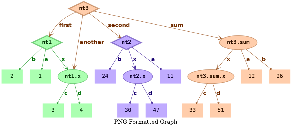
If you do not need svg format, you can dump it to png format like this
1 2 3 4 5 | treevalue graph \ -t 'node_share_demo.*' \ -o 'shared_nodes.dat.png' \ -T 'PNG Formatted Graph' \ -c 'bgcolor=#ffffff00' |
The dumped graph shared_nodes.dat.png should be like this, its format is png.
Besides, if the graphviz code (gv format) is just all what you need, you can dump the gv source code with the following command line.
1 2 3 4 5 | treevalue graph \ -t 'node_share_demo.*' \ -o 'shared_nodes.dat.gv' \ -T 'PNG Formatted Graph' \ -c 'bgcolor=#ffffff00' |
The dumped source code shared_nodes.dat.gv should be like this
1 2 3 4 5 6 7 8 9 10 11 12 13 14 15 16 17 18 19 20 21 22 23 24 25 26 27 28 29 30 31 32 33 34 35 36 37 38 39 40 41 42 | // PNG Formatted Graph digraph png_formatted_graph { graph [bgcolor="#ffffff00" label="PNG Formatted Graph"] node_7f1a95c77820 [label=nt1 color="#3eb24899" fillcolor="#73ff7e99" fontcolor="#003304ff" fontname="monospace bold" penwidth=3 shape=diamond style=filled] node_7f1a95c778b0 [label=nt2 color="#5b3eb299" fillcolor="#9673ff99" fontcolor="#0d0033ff" fontname="monospace bold" penwidth=3 shape=diamond style=filled] node_7f1a95c779d0 [label=nt3 color="#b26f3e99" fillcolor="#ffad7399" fontcolor="#331500ff" fontname="monospace bold" penwidth=3 shape=diamond style=filled] value__node_7f1a95c77820__a [label=1 color="#3eb24800" fillcolor="#73ff7e99" fontcolor="#003304ff" fontname=monospace penwidth=1.5 shape=box style=filled] node_7f1a95c77820 -> value__node_7f1a95c77820__a [label=a arrowhead=dot arrowsize=0.5 color="#1f9929cc" fontcolor="#00730aff" fontname="Times-Roman bold"] value__node_7f1a95c77820__b [label=2 color="#3eb24800" fillcolor="#73ff7e99" fontcolor="#003304ff" fontname=monospace penwidth=1.5 shape=box style=filled] node_7f1a95c77820 -> value__node_7f1a95c77820__b [label=b arrowhead=dot arrowsize=0.5 color="#1f9929cc" fontcolor="#00730aff" fontname="Times-Roman bold"] node_7f1a95c777f0 [label="nt1.x" color="#3eb24899" fillcolor="#73ff7e99" fontcolor="#003304ff" fontname="monospace bold" penwidth=1.5 shape=ellipse style=filled] node_7f1a95c77820 -> node_7f1a95c777f0 [label=x arrowhead=vee arrowsize=1.0 color="#1f9929cc" fontcolor="#00730aff" fontname="Times-Roman bold"] value__node_7f1a95c778b0__a [label=11 color="#5b3eb200" fillcolor="#9673ff99" fontcolor="#0d0033ff" fontname=monospace penwidth=1.5 shape=box style=filled] node_7f1a95c778b0 -> value__node_7f1a95c778b0__a [label=a arrowhead=dot arrowsize=0.5 color="#3d1f99cc" fontcolor="#1d0073ff" fontname="Times-Roman bold"] value__node_7f1a95c778b0__b [label=24 color="#5b3eb200" fillcolor="#9673ff99" fontcolor="#0d0033ff" fontname=monospace penwidth=1.5 shape=box style=filled] node_7f1a95c778b0 -> value__node_7f1a95c778b0__b [label=b arrowhead=dot arrowsize=0.5 color="#3d1f99cc" fontcolor="#1d0073ff" fontname="Times-Roman bold"] node_7f1a95c77970 [label="nt2.x" color="#5b3eb299" fillcolor="#9673ff99" fontcolor="#0d0033ff" fontname="monospace bold" penwidth=1.5 shape=ellipse style=filled] node_7f1a95c778b0 -> node_7f1a95c77970 [label=x arrowhead=vee arrowsize=1.0 color="#3d1f99cc" fontcolor="#1d0073ff" fontname="Times-Roman bold"] node_7f1a95c779d0 -> node_7f1a95c77820 [label=first arrowhead=vee arrowsize=1.0 color="#99521fcc" fontcolor="#733000ff" fontname="Times-Roman bold"] node_7f1a95c779d0 -> node_7f1a95c778b0 [label=second arrowhead=vee arrowsize=1.0 color="#99521fcc" fontcolor="#733000ff" fontname="Times-Roman bold"] node_7f1a95c779d0 -> node_7f1a95c777f0 [label=another arrowhead=vee arrowsize=1.0 color="#99521fcc" fontcolor="#733000ff" fontname="Times-Roman bold"] node_7f1a95c77850 [label="nt3.sum" color="#b26f3e99" fillcolor="#ffad7399" fontcolor="#331500ff" fontname="monospace bold" penwidth=1.5 shape=ellipse style=filled] node_7f1a95c779d0 -> node_7f1a95c77850 [label=sum arrowhead=vee arrowsize=1.0 color="#99521fcc" fontcolor="#733000ff" fontname="Times-Roman bold"] value__node_7f1a95c777f0__c [label=3 color="#3eb24800" fillcolor="#73ff7e99" fontcolor="#003304ff" fontname=monospace penwidth=1.5 shape=box style=filled] node_7f1a95c777f0 -> value__node_7f1a95c777f0__c [label=c arrowhead=dot arrowsize=0.5 color="#1f9929cc" fontcolor="#00730aff" fontname="Times-Roman bold"] value__node_7f1a95c777f0__d [label=4 color="#3eb24800" fillcolor="#73ff7e99" fontcolor="#003304ff" fontname=monospace penwidth=1.5 shape=box style=filled] node_7f1a95c777f0 -> value__node_7f1a95c777f0__d [label=d arrowhead=dot arrowsize=0.5 color="#1f9929cc" fontcolor="#00730aff" fontname="Times-Roman bold"] value__node_7f1a95c77970__c [label=30 color="#5b3eb200" fillcolor="#9673ff99" fontcolor="#0d0033ff" fontname=monospace penwidth=1.5 shape=box style=filled] node_7f1a95c77970 -> value__node_7f1a95c77970__c [label=c arrowhead=dot arrowsize=0.5 color="#3d1f99cc" fontcolor="#1d0073ff" fontname="Times-Roman bold"] value__node_7f1a95c77970__d [label=47 color="#5b3eb200" fillcolor="#9673ff99" fontcolor="#0d0033ff" fontname=monospace penwidth=1.5 shape=box style=filled] node_7f1a95c77970 -> value__node_7f1a95c77970__d [label=d arrowhead=dot arrowsize=0.5 color="#3d1f99cc" fontcolor="#1d0073ff" fontname="Times-Roman bold"] value__node_7f1a95c77850__a [label=12 color="#b26f3e00" fillcolor="#ffad7399" fontcolor="#331500ff" fontname=monospace penwidth=1.5 shape=box style=filled] node_7f1a95c77850 -> value__node_7f1a95c77850__a [label=a arrowhead=dot arrowsize=0.5 color="#99521fcc" fontcolor="#733000ff" fontname="Times-Roman bold"] node_7f1a95c779a0 [label="nt3.sum.x" color="#b26f3e99" fillcolor="#ffad7399" fontcolor="#331500ff" fontname="monospace bold" penwidth=1.5 shape=ellipse style=filled] node_7f1a95c77850 -> node_7f1a95c779a0 [label=x arrowhead=vee arrowsize=1.0 color="#99521fcc" fontcolor="#733000ff" fontname="Times-Roman bold"] value__node_7f1a95c77850__b [label=26 color="#b26f3e00" fillcolor="#ffad7399" fontcolor="#331500ff" fontname=monospace penwidth=1.5 shape=box style=filled] node_7f1a95c77850 -> value__node_7f1a95c77850__b [label=b arrowhead=dot arrowsize=0.5 color="#99521fcc" fontcolor="#733000ff" fontname="Times-Roman bold"] value__node_7f1a95c779a0__c [label=33 color="#b26f3e00" fillcolor="#ffad7399" fontcolor="#331500ff" fontname=monospace penwidth=1.5 shape=box style=filled] node_7f1a95c779a0 -> value__node_7f1a95c779a0__c [label=c arrowhead=dot arrowsize=0.5 color="#99521fcc" fontcolor="#733000ff" fontname="Times-Roman bold"] value__node_7f1a95c779a0__d [label=51 color="#b26f3e00" fillcolor="#ffad7399" fontcolor="#331500ff" fontname=monospace penwidth=1.5 shape=box style=filled] node_7f1a95c779a0 -> value__node_7f1a95c779a0__d [label=d arrowhead=dot arrowsize=0.5 color="#99521fcc" fontcolor="#733000ff" fontname="Times-Roman bold"] } |
Or if you need to put it to the stdout, you can do like this
1 2 3 4 5 | treevalue graph \ -t 'node_share_demo.*' \ -O \ -T 'PNG Formatted Graph' \ -c 'bgcolor=#ffffff00' |
The output in stdout should almost the same like the source code file shared_nodes.dat.gv.
Note
When -O option is used, the -o will be ignored.
Reuse the Value Nodes
In some cases, the values in the trees’ nodes is the same object (using the same memory id). So it’s better to put them together in the dumped graph.
For example, in the python code file share_demo.py
1 2 3 4 5 6 7 8 9 10 11 12 13 14 15 16 17 18 | import numpy as np from treevalue import FastTreeValue st1 = FastTreeValue({ 'a': 1, 'b': [1, 2], 'x': { 'c': 3, 'd': np.zeros((3, 2)), } }) st2 = FastTreeValue({ 'np': st1.x.d, 'ar': st1.b, 'a': st1.a, 'arx': [1, 2], }) |
You can run the following command
1 2 3 4 5 | treevalue graph \ -t 'share_demo.*' \ -o 'no_shared_values.dat.svg' \ -T 'No Shared Values' \ -c 'bgcolor=#ffffff00' |
The dumped graph no_shared_values.dat.svg should be like this, all the value nodes are separated in the default options.

We can solve this problem by adding -D option in the command, which means duplicate all the value nodes.
1 2 3 4 5 6 | treevalue graph \ -t 'share_demo.*' \ -o 'shared_all_values.dat.svg' \ -T 'Shared All Values' \ -c 'bgcolor=#ffffff00' \ -D |
In the dumped graph shared_all_values.dat.svg, all the value nodes with the same id are put together.

Note
When -D is used, all the values in leaf node with the same id will share exactly one leaf node in the dumped graph.
But actually in python, most of the basic data types are immutable, which means all the 1 in python code are actually the same object, for their ids are the same. So in the image shared_all_values.dat.svg, even the leaf node 1 are shared.
This phenomenon may reduce the intuitiveness of the image in many cases. Please notice this when you are deciding to use -D option.
Because of the problem mentioned in the note above, in most of the cases, it’s a better idea to use -d option to assign which types should be duplicated and which should not. Like the example below.
1 2 3 4 5 6 | treevalue graph \ -t 'share_demo.*' \ -o 'shared_values.dat.svg' \ -T 'Shared Values' \ -c 'bgcolor=#ffffff00' \ -d list -d numpy.ndarray |
The dumped graph shared_values.dat.svg should be like this, the 1 is not duplicated any more, but list and np.ndarray will be duplicated.
